Absorption of the solar flux

Theory

Before reaching the D-region, the solar fluxes are absorbed by the neutral constituent of the atmosphere at higher altitudes. Thus, the flux at an altitude \(z\) is written

\[\begin{split}F(\lambda, z) &= F(\lambda, \infty) \times \exp\left(-\sum_i \sigma_i^a \int n_i ds \right) \\ &= F(\lambda, \infty) \times \exp(-\tau)\end{split}\]

where the sum on \(i\) is a sum over all neutral species, \(ds\) is the infinetisimal distance travelled by the flux, and \(\sigma_i^a\) is the absorption cross-section of species \(i\) at wavelength \(\lambda\). \(F(z)\) is the absorbed flux while \(F(\infty)\) is the solar flux (e.g. [singer1961] ).

Instead of computing the integral on \(ds\), the use of the Chapman function allows it to be computed on \(dz\):

\[\begin{split}\tau &= Ch(X, \chi) \sum_i \int_z^\infty \sigma_i^a n_i dz \\ &= Ch(X, \chi) H \sigma_i^a n_i(z)\end{split}\]

where \(\chi\) is the solar zenith angle, \(Ch\) is the Chapman function and \(X\) is the ratio of the Earth radius and the altitude with respect to the atmosphere scale height \(H\) (e.g. [brasseur2005] )

The values of \(\sigma^a\) comes from [siskind2022] for the HXR flux, [solomon2005] for the SXR flux and [reddmann2003] for the absorption of Lyman-a flux.

Practice

In practice, the first thing that needs to be computed is the ionosphere scale height \(H\). It is simply given by

\[H = \frac{k T_n}{g M}\]

where \(T_n\) is the neutral temperature and \(M\) is the average particule mass. This computation is done through the compute_H() function.

H = compute_H(neutrals_here)

Then, the Chapman function for solar zenith angle \(\chi\) is evaluated, following the approximation by [smith1972] .

Ch, H = chapman(chi, neutrals_here)

Note

\(H\) is actually computed inside the chapman() function, and returned by this function

\(\tau\) is computed through the get_tau() function (which also calls chapman()). To perform this, the absorption cross-sections of the main neutral species are needed. Those are taken from Table 1 of [pavlov2014] and references therein. This function returns \(\tau\) at altitude \(z\) specified as input.

\(\tau\) over all altitudes in the D-region is computed by the compute_tau(). This is done during the initialisation of the radiation class, since this may be done as soon as the solar fluxes are known and the neutral densities initialised.

tau_EUV, tau_SXR, tau_HXR = cs.compute_tau(self, neutrals_here, chi)

We only consider three radiations wavelengths here, the soft solar X-rays, the hard X-rays and the Lyman-\(\alpha\) radiation.

Results

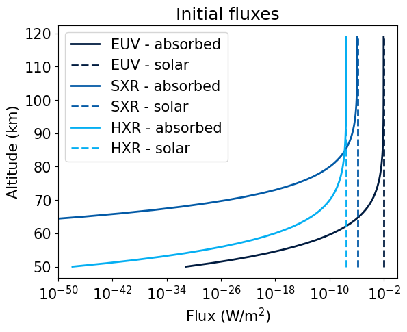
Here are an example of results for a quiet period, over the NSY transmitter in November 2023 (\(\chi = 58°\)).

Another way to look at this is to plot the transmittion factor, which is the term \(\exp(-\tau)\).

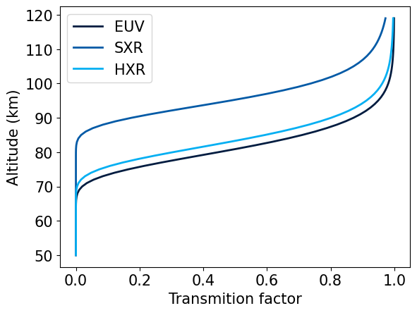
This matches Figure 25 (p 186) of Physics of the Upper Atmosphere by Ratcliffe (1960)

HXR

On the figure above, it is visible that the SXR do not reach the D-region altitudes. Similarly, the HXR only reach to an altitude of 70 km.

Though the fact that the SXR do not participate in the D-region was already noted ([ratcliffe1960], [barta2019]), the HXR do impact the D-region. However, to see their effect on the lower altitudes, it is necessary to discretise the HXR band as given by GOES:

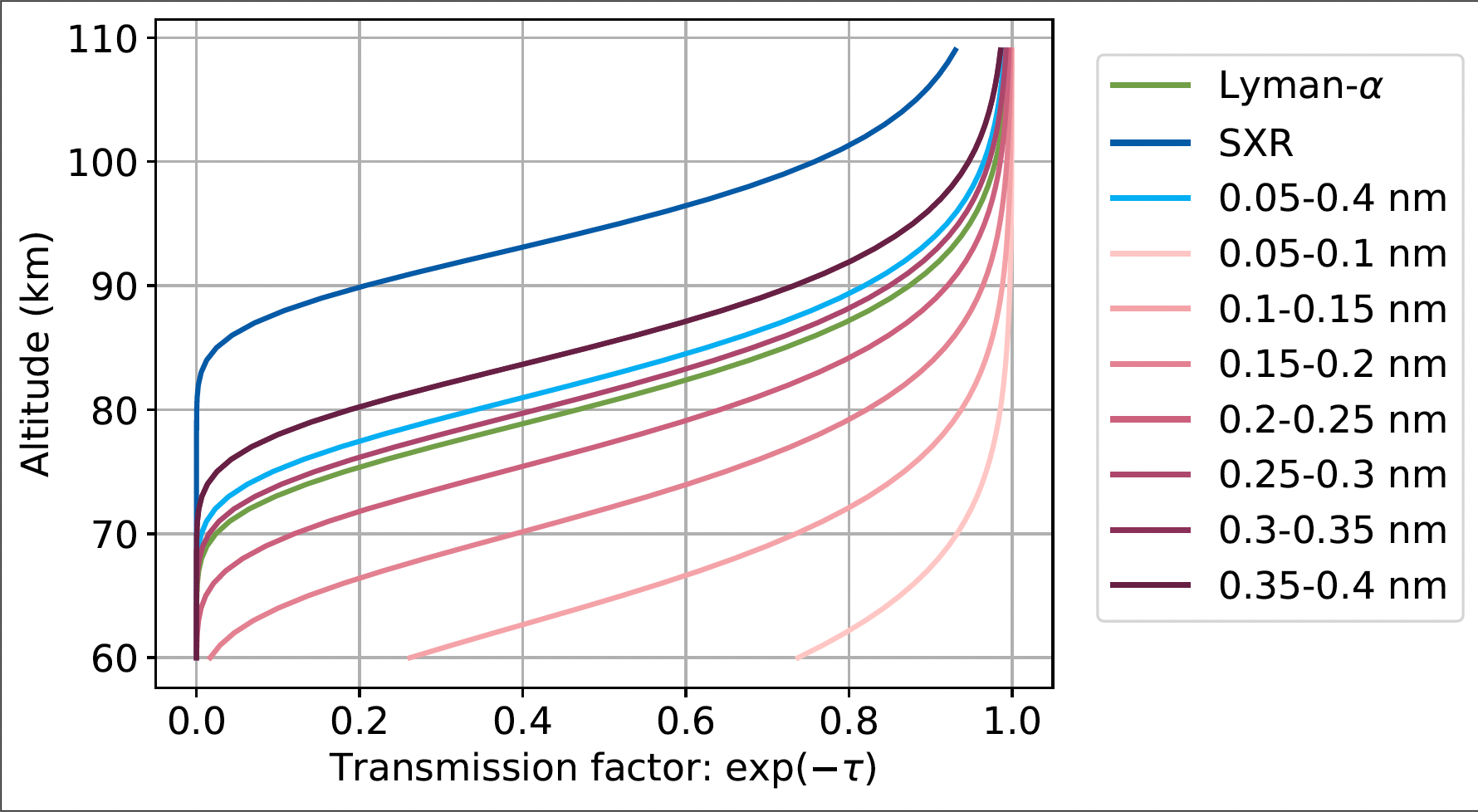
Taking this ionisation into account thus requires discretising the HXR band. We bin it in 0.05 nm wide windows, following [siskind2022] . To do this, full codes such as NRLFLARES or FISM may be used. However, in the interest of speed and to provide a full code, we here suppose that the HXR bands are divided into two regions:

1. 0.05-0.15 nm, during which the flux linearly increases by a factor 100

2. 0.15-0.4 nm during which it linearly increases by a factor 5

This is very approximate, but may be corrected in the future..