Initialisation of ions

The ions are ionised by the different sources presented in Photoionisation of neutral species. For those processes, the different cross sections and ionisation rates are rather well-known (e.g. [pavlov2014] ). However, the main unknown is the concentration of [NO]. Over the years, different models or measurements gave different estimates, from \(5\times10^5 \text{cm}^{-3}\) [rusch1981] to \(10^9 \text{cm}^{-3}\) [pearce1969] .

In Neutral densities, we described a scheme by [mitra1966] to initialise \([NO]\). This parametrisation gives the correct shape for \(NO\), but not necessarily the correct value. Since this is our last unknown, we proceed as follows.

First initialisation of ions

The ions are initalised a first time, assuming the \(NO\) density given by [mitra1966]. The scheme doesn’t need to be run until it stabilises, which may take some time. Instead, we can run it for a few seconds, until it approaches a stable solution:

import lir_achem.compute_coefficients_mitra as ccm
import lir_achem.mitra_rowe_scheme as mrs

# Compute photon fluxes, using the taus already computed
Phi_SXR, Phi_HXR, Phi_EUV = ci.compute_photon_flux(rad_here)

# Load the chemistry coefficients

coefficients = ccm.get_mr_coeffs(n_here, e_here)

# Initial conditions - Everything is 0, except fluxes
zero_density = np.zeros(np.shape(e_here.densities))
densities = np.hstack(
    (
        zero_density,
        zero_density,
        zero_density,
        zero_density,
        zero_density,
        zero_density,
        zero_density,
        Phi_SXR,
        Phi_HXR,
    )
)

sol = solve_ivp(
mrs.chemistry_mr_eq,
[0, 40],
densities,
args=(coefficients, rad_here, n_here, Phi_EUV, False, today),
)

# Get everything in the right format
length_one_density = int(np.size(e_here.densities))
Ne = sol.y[0:length_one_density, :]
O2m = sol.y[length_one_density : 2 * length_one_density, :]
Xm = sol.y[2 * length_one_density : 3 * length_one_density, :]
NOp = sol.y[3 * length_one_density : 4 * length_one_density, :]
Yp = sol.y[4 * length_one_density : 5 * length_one_density, :]
O2p = sol.y[5 * length_one_density : 6 * length_one_density, :]
O4p = sol.y[6 * length_one_density : 7 * length_one_density, :]
time_sol = sol.t

This gives the different results below:

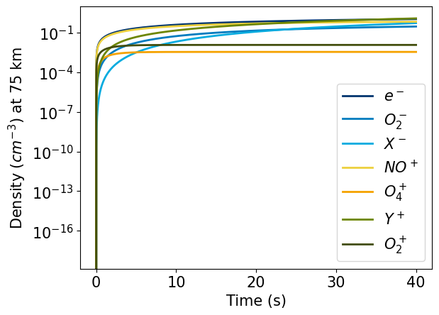
Variations of the densities with time

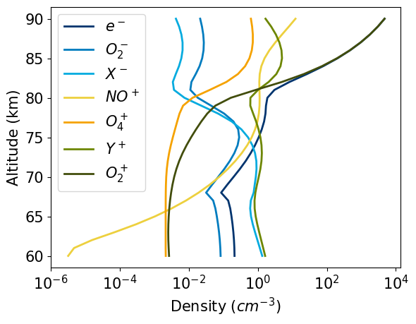
Final ion profiles after the first initialisation

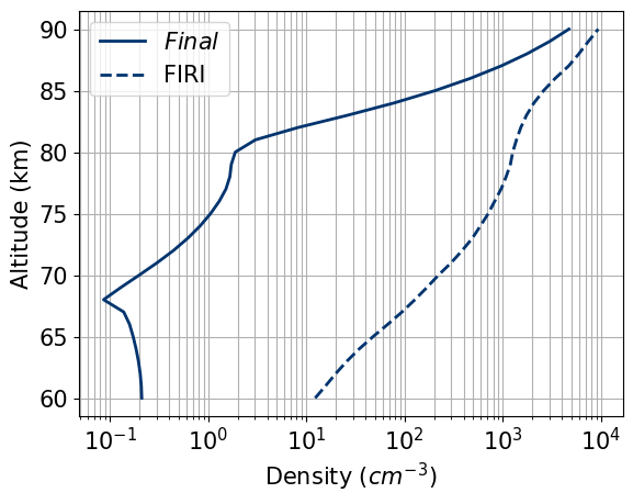
Comparison between the final electron density and the results from FIRI

Second initialisation of ions

As seen just above, after this first initialisation, the electron profile is quite far to the results from the FIRI model, especially at middle altitudes and low altitudes in the D-region, where most electrons come from the ionisation of \([NO]\). Because the largest unknown here is \([NO]\), we compute the difference between the our value of \(N_e\) at 75 km and the one obtained from FIRI. We then multiply this factor to the density of \([NO]\) that we had. With this new value of \([NO]\), the ions may be initialised again (from 0). This time however, the model needs to run longer, until the different species stabilise.

# We compute the ionisation that would be needed to reach the FIRI electron density
alpha = e_here.densities[id] / Ne[id, -1]
n_here.NO = n_here.NO * alpha

# Re-do the initialisation with the new NO

# Load the chemistry coefficients
coefficients = ccm.get_mr_coeffs(n_here, e_here)

# Initial conditions
zero_density = np.zeros(np.shape(e_here.densities))
densities = np.hstack(
    (
        zero_density,
        zero_density,
        zero_density,
        zero_density,
        zero_density,
        zero_density,
        zero_density,
        Phi_SXR,
        Phi_HXR,
    )
)

sol = solve_ivp(
    mrs.chemistry_mr_eq,
    [0, 4e3],
    densities,
    args=(coefficients, rad_here, n_here, Phi_EUV, False, today),
)

# Get everything in the right format
length_one_density = int(np.size(e_here.densities))
Ne = sol.y[0:length_one_density, :]
O2m = sol.y[length_one_density : 2 * length_one_density, :]
Xm = sol.y[2 * length_one_density : 3 * length_one_density, :]
NOp = sol.y[3 * length_one_density : 4 * length_one_density, :]
Yp = sol.y[4 * length_one_density : 5 * length_one_density, :]
O2p = sol.y[5 * length_one_density : 6 * length_one_density, :]
O4p = sol.y[6 * length_one_density : 7 * length_one_density, :]
time_sol = sol.t

Tip

To check whether the densities have indeed stabilised, you can plot the negative charge surplus. Normally it should be very close to 0 compared to the densities modeled.

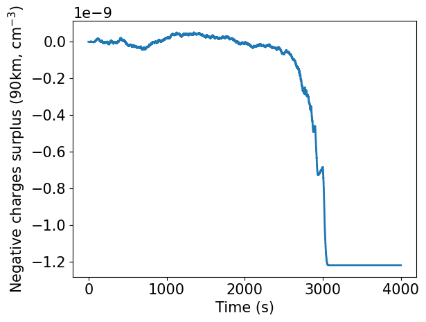
In this image for example, the surplus of negative charges is very low. However, it varies a little before 3000 s, before suddently stabilising when the different ion densities reach their quiet values. This should always be checked, except for the first ion initialisation for which we do not seek stable values, just densities close to their quiet values.

Once this is done, the electron density is much closer to FIRI electron densities at all altitudes:

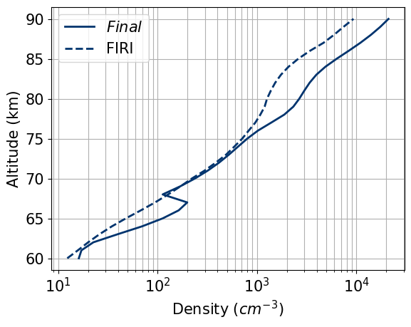
We can also check the different results, and compare them to publish litterature (e.g. [reid1979] )

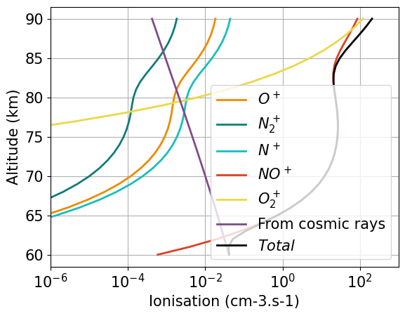
Ionisation sources in quiet time

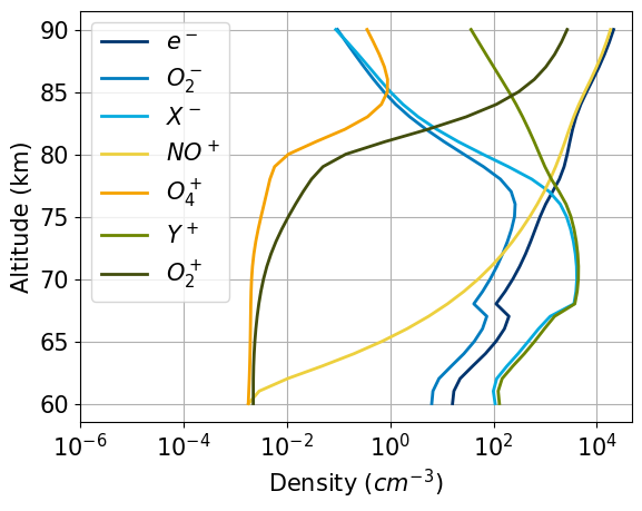
Variation of the different ion species with altitude

The \(NO\) density also match previous estimates:

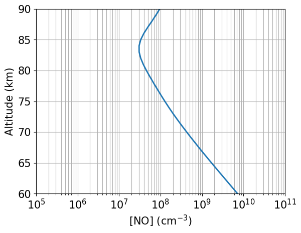
Variation of \([NO]\) with altitudes after the second ion initialisation